Conjugates¶

conjugates are types equivalent to likelihood-prior pairs in Bayesian paradigm. They comprise of a likelihood distribution and a prior distribution where the parameters of the likelihood are drawn from the prior. Apart from the parameters of the likelihood and the prior distributions, a conjugate component also contains the data points which are associated with it.

All conjugates provided in this package are organized in a type hierarchy as follows:

abstract Conjugates
conjugate <: Conjugates

Conjugates names follow the convention of LikelihoodPrior. Therefore MultinomialDirichlet is a Bayesian conjugate component with a Multinomial likelihood where the Multinomial distribution parameter is drawn from Dirichelt distribution.

Conjugate distributions¶

Here is a list of implemented conjugates. This list will grow as I continue to develop this package.

Gaussian1DGaussian1D
MultinomialDirichlet

Gaussian1DGaussian1D¶

It is a conjugate component with univariate Gaussian likelihood. The variance of the likelihood is known. The mean parameter of the likelihood is drawn from another univariate Gaussian distribution.

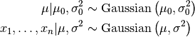
$\mu|\mu_{0},\sigma_{0}^{2} &\sim \text{Gaussian}\left(\mu_{0},\sigma_{0}^{2}\right) \\ x_{1},\ldots,x_{n}|\mu,\sigma^{2} &\sim \text{Gaussian}\left(\mu,\sigma^{2}\right)$

It is parametrized by the mean and variance of the prior, m0 and v0, and the variance of the likelihood vv.

julia> qq = Gaussian1DGaussian1D(m0, v0, vv)

julia> qq = Gaussian1DGaussian1D(2, 10, 0.5)
Gaussian1DGaussian1D conjugate component
likelihood parameters: mu=2.0, vv=0.5
prior parameters     : m0=2.0, v0=10.0
number of data points: nn=0

MultinomialDirichlet¶

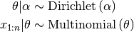
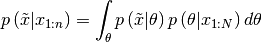
It is a conjugate component with Multinmomial likelihood where the likelihood parameter (i.e. Multinomial vector) is drawn from a Dirichlet distirbution.

$\theta|\alpha &\sim \text{Dirichlet}\left(\alpha\right)\\ x_{1:n}|\theta &\sim \text{Multinomial}\left(\theta\right)$

where $\theta=\left[\theta_{1},\ldots,\theta_{K}\right]$ and $\alpha=\left[\alpha_{1},\ldots,\alpha_{K}\right]$ . It is parametrized by the Dirichlet concentration parametr. You can create a MultinomialDirichlet object by passing the cardinality and prior concentration parameter.

julia> qq = MultinomialDirichlet(5, 2.0)
MultinomialDirichlet component
cardinality: dd=5, Dirichlet prior parameter: aa=0.4
data: mm=0, nn=0

Note

write a few sentences about nn and mm and the two different forms that Multinomial Dirichelty can be used.

Interface¶

In this section the functions that operate on conjugates are described.

Adding and removing data points¶

Note

Since these functions are not meant to be used directly by the user, they are not exported.

Use additem! or delitem! functions to add or delete a data point.

julia> qq = Gaussian1DGaussian1D(2, 10, 0.5)
Gaussian1DGaussian1D conjugate component
likelihood parameters: mu=2.0, vv=0.5
prior parameters     : m0=2.0, v0=10.0
number of data points: nn=0

julia> BIAS.additem!(qq, 3.0)
julia> BIAS.additem!(qq, 3.5)
julia> BIAS.additem!(qq, 2.8)
likelihood parameters: mu=3.099999.0, vv=0.5
prior parameters     : m0=2.0, v0=10.0
number of data points: nn=3

julia> BIAS.delitem!(qq, 2.8)
Gaussian1DGaussian1D conjugate component
likelihood parameters: mu=3.249999, vv=0.5
prior parameters     : m0=2.0, v0=10.0
number of data points: nn=2

Posterior distribution¶

Use posterior to find the posterior probability distribution of the likelihood parameters given the observations. Since we use conjugate priors, the posterior will have the same form as prior.

$p\left(\theta|x_{1:n}\right)\propto p\left(\theta\right)p\left(x_{1:n}|\theta\right)$

julia> qq = Gaussian1DGaussian1D(2, 10, 0.5)
julia> BIAS.additem!(qq, 3.0)
julia> BIAS.additem!(qq, 3.5)
julia> BIAS.additem!(qq, 2.8)
likelihood parameters: mu=3.099999.0, vv=0.5
prior parameters     : m0=2.0, v0=10.0
number of data points: nn=3

julia> posterior(qq)
Gaussian1D distribution
mean: mu=3.081967, variance: vv=0.163934

Posterior predictive likelihood¶

Note

Since these functions are not meant to be used directly by the user, they are not exported.

Use logpredictive to compute the posterior predictive likelihood of a component given a data point.

$p\left(\tilde{x}|x_{1:n}\right)=\int_{\theta}p\left(\tilde{x}|\theta\right)p\left(\theta|x_{1:N}\right)d\theta$

julia> qq = Gaussian1DGaussian1D(2, 10, 0.5)
julia> BIAS.additem!(qq, 3.0)
julia> BIAS.additem!(qq, 3.5)
julia> BIAS.additem!(qq, 2.8)
julia> posterior(qq)
Gaussian1D distribution
mean: mu=3.081967, variance: vv=0.163934

julia> BIAS.logpredictive(qq, 3.2)
-0.724644
julia> BIAS.logpredictive(qq, 4.2)
-1.655550