BMM for univariate Gaussian likelihood¶

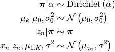
Here we look at the problem of fitting a Bayesian Mixture Model to a series of data points that are drawn from a number of Gaussian distributions. We assume:

the variance of these Gaussian components is fixed and known
the mean of these Gaussian components are drawn from another Gaussian distribution

What we are looking for is the mean of inferred Gaussian components after observing the data.

Problem¶

We have $N$ data points generated by $K$ univariate Gaussian distributions with known variance and unknown means. Infer the means from the data.

Model¶

$\boldsymbol{\pi}|\alpha &\sim \text{Dirichlet}\left(\alpha\right)\\ \mu_{k}|\mu_{0},\sigma_{0}^{2} &\sim \mathcal{N}\left(\mu_{0},\sigma_{0}^{2}\right)\\ z_{n}|\boldsymbol{\pi} &\sim \boldsymbol{\pi}\\ x_{n}|z_n,\mu_{1:K},\sigma^{2} &\sim \mathcal{N}\left(\mu_{z_{n}},\sigma^{2}\right)$

Solution¶

Simulate the data¶

First we need to simulate a dataset. For this, we have to specify the parameters of some “true” clusters and use the generative process mentioned above to obtain the observations. Each cluster is specified with a univariate Gaussian distribution. Below, we assume 5 Gaussian distributions with means [1, 2, 3, 4, 5] and variance equal to 0.01. The total number of observations is 500.

using BIAS
srand(123)

true_KK = 5                             # number of components
NN = 500                                # number of data points

vv = 0.01                                # fixed variance
true_atoms = [Gaussian1D(kk, vv) for kk = 1:true_KK]

mix = ones(Float64, true_KK)/true_KK
xx = ones(Float64, NN)
true_zz = ones(Int, NN)
true_nn = zeros(Int, true_KK)

for n=1:NN
    kk = BIAS.sample(mix)
    true_zz[n] = kk
    xx[n] = sample(true_atoms[kk])
    true_nn[kk] += 1
end

Let’s look at the true cluster parameters. true_nn[kk] shows the number of data points generate by cluster kk.

julia> true_atoms
5-element Array{BIAS.Gaussian1D,1}:
 Gaussian1D distribution
mean: mu=1.0, variance: vv=0.1

 Gaussian1D distribution
mean: mu=2.0, variance: vv=0.1

 Gaussian1D distribution
mean: mu=3.0, variance: vv=0.1

 Gaussian1D distribution
mean: mu=4.0, variance: vv=0.1

 Gaussian1D distribution
mean: mu=5.0, variance: vv=0.1

julia> true_nn
5-elemet Array{Int64, 1}
 102
  88
 116
  99
  95

Model construction¶

The prior-likelihood pair of this model can be seen as a Gaussian1DGaussian1D component.

m0 = mean(xx)
v0 = 2.0
q0 = Gaussian1DGaussian1D(m0, v0, vv)

Now we construct and instantiate the model:

KK = true_KK
bmm_aa = 1.0
bmm = BMM(q0, KK, bmm_aa)

zz = zeros(Int64, length(xx))
init_zz!(bmm, zz)

Inferecne¶

Now it is time to run the inference routine:

n_burnins   = 100
n_lags      = 2
n_samples   = 200
store_every = 100
filename    = "demo_BMM_Gaussian1DGaussian1D_"

collapsed_gibbs_sampler!(bmm, xx, zz, n_burnins, n_lags, n_samples, store_every, filename)

to obtain the posterior distributions:

julia> posterior_components, nn = posterior(bmm, xx, zz)
julia> posterior_components
5-element Array{BIAS.Gaussian1D,1}:
 Gaussian1D distribution
mean: mu=4.990567102836185, variance: vv=0.00010525761802010421

 Gaussian1D distribution
mean: mu=3.00416499910953, variance: vv=8.620318089737512e-5

 Gaussian1D distribution
mean: mu=1.9939209647504217, variance: vv=0.00011362990739162548

 Gaussian1D distribution
mean: mu=1.0153304673990435, variance: vv=9.803441007793736e-5

 Gaussian1D distribution
mean: mu=4.000720712951586, variance: vv=0.00010100499974748751

julia> nn
5-element Array{Int64,1}:
  95
 116
  88
 102
 99

As it is readily seen nn is equal to true_nn by permutation and the posterior distribution of clusters are very close to true_atoms.