BMM for Multinomial likelihood¶

Here we look at the problem of fitting a Bayesian mixture model to a series of observations made from Multinomial distributions.

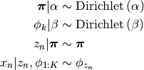
Here we assume:

the probability vector of the Multinomial distribution is drawn from a Dirichlet distribution

Problem¶

We have $N$ observation generated by $K$ Multinomial distributions (i.e. topics). Infer the topics from the data.

Model¶

$\boldsymbol{\pi}|\alpha &\sim \text{Dirichlet}\left(\alpha\right)\\ \phi_{k}|\beta &\sim \text{Dirichlet}\left(\beta\right)\\ z_{n}|\boldsymbol{\pi} &\sim \boldsymbol{\pi}\\ x_{n}|z_{n}, \phi_{1:K} &\sim \phi_{z_{n}}$

Solution¶

Simulate the data¶

First we need to simulate a dataset. For this, we have to specify the parameters of some “true” mixture components and use the generative process mentioned above, to obtain the observations. Each component is a Multinomial distribution over a vocabulary that we call it a topic. Below, we create 4 topics over 25 words.

using BIAS
srand(123)

true_KK    = 4
vocab_size = 25

true_topics = BIAS.gen_bars(true_KK, vocab_size, 0.0)
4x25 Array{Float64,2}:
0.2  0.0  0.0  0.0  0.0  0.2  0.0  0.0  0.0  0.0  …  0.0  0.0  0.0  0.0  0.2  0.0  0.0  0.0  0.0
0.0  0.2  0.0  0.0  0.0  0.0  0.2  0.0  0.0  0.0     0.2  0.0  0.0  0.0  0.0  0.2  0.0  0.0  0.0
0.2  0.2  0.2  0.2  0.2  0.0  0.0  0.0  0.0  0.0     0.0  0.0  0.0  0.0  0.0  0.0  0.0  0.0  0.0
0.0  0.0  0.0  0.0  0.0  0.2  0.2  0.2  0.2  0.2     0.0  0.0  0.0  0.0  0.0  0.0  0.0  0.0  0.0

Looking at the numerical values of the topics is not very convenient. Instead we can think of each topic as a 5x5 image and plot it.

../_images/demo_BMM_MultinomialDirichlet_true.png

true topics

Now we are ready to draw observations from the simulated topics. We assume each observation is a sentence with 15 words. We have 200 observations in total.

n_sentences = 200
n_tokens    = 15

mix = ones(true_KK) / true_KK
xx = Array(Sent, n_sentences)
true_zz = zeros(Int, n_sentences)
true_nn = zeros(Int, true_KK)
for ii = 1:n_sentences
    kk = sample(mix)
    true_zz[ii] = kk
    true_nn[kk] += 1
    sentence = sample(true_topics[kk, :][:], n_tokens)
    xx[ii] = BIAS.sparsify_sentence(sentence)
end

xx is a vector of type Sent.

julia> xx[1]
BIAS.Sent([10,9,7,8,6],[2,3,4,3,3])

Model construction¶

The prior-likelihood pair of this model can be seen as a MultinomialDirichlet component.

d = vocab_size
aa = 1.0
q0 = MultinomialDirichlet(dd, aa)

Now we construct and instantiate the model:

bmm_KK = true_KK
bmm_aa = 0.1
bmm = BMM(q0, bmm_KK, bmm_aa)

# Sampling
zz = zeros(Int, length(xx))
init_zz!(bmm, zz)

Inferecne¶

Now it is time to run the inference routine:

n_burnins   = 100
n_lags      = 2
n_samples   = 200
store_every = 100
filename    = "demo_BMM_MultinomialDirichlet_"

collapsed_gibbs_sampler!(bmm, xx, zz, n_burnins, n_lags, n_samples, store_every, filename)

to obtain the posterior distributions:

posterior_components, nn = posterior(bmm, xx, zz)
inferred_topics = zeros(Float64, bmm.K, vocab_size)
for kk = 1:length(posterior_components)
    inferred_topics[kk, :] = mean(posterior_components[kk])
end

visualize_bartopics(inferred_topics)

../_images/demo_BMM_MultinomialDirichlet_posterior.png

inferred topics

As it is readily seen from two figures, the model has successfully inferred the topics. Also:

julia> true_nn
4-element Array{Int64, 1}
 51
 55
 49
 45

julia> nn
4-element Array{Int64, 1}
 49
 51
 55
 45