LDA for univariate Gaussian likelihood¶

We have already looked at the problem of modeling a group of data points that are drawn from a mixture of Gaussian distributions in BMM for univariate Gaussian likelihood. This is the simplest case of Bayesian mixture modeling. Now what if instead of one group of data points, we have J groups? This adds one level of hierarchy on the representation of the data that needs to be addressed in the model as well. LDA was proposed to solve this problem.

Here we Here we look at the problem of modeling J groups of data points where each grouop is generated by a mixture of Gaussian distributions where it is desired that groups share their mixing components.

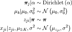
We assume:

the variance of these Gaussian components is fixed and known
the mean of these Gaussian components are drawn from another Gaussian distribution

What we are looking for is the mean of inferred Gaussian components after observing the data.

Problem¶

We have $J$ groups of data points. Each group is generated by a mixture of $K$ univariate Gaussian distributions with known variance and unknown means. Assuming J groups share their mixing components, infer the unknown means from the data.

Model¶

$\boldsymbol{\pi}_{j}|\alpha &\sim \text{Dirichlet}\left(\alpha\right)\\ \mu_{k}|\mu_{0},\sigma_{0}^{2} &\sim \mathcal{N}\left(\mu_{0},\sigma_{0}^{2}\right)\\ z_{ji}|\boldsymbol{\pi} &\sim \boldsymbol{\pi}\\ x_{ji}|z_{ji}, \mu_{1:K},\sigma^{2} &\sim \mathcal{N}\left(\mu_{z_{ji}},\sigma^{2}\right)$

Solution¶

Simulate the data¶

First we need to simulate a dataset. For this, we have to specify the parameters of some “true” mixture components and then use the generative process mentioned above to obtain the observations. Each component is a univariate Gaussian distribution. Below, we assume 5 Gaussian distributions with means [1, 2, 3, 4, 5] and variance equal to 0.01.

using BIAS
srand(123)

true_KK = 5                                # number of components
vv = 0.01                                  # fixed variance
true_atoms = [Gaussian1D(kk, vv) for kk = 1:true_KK]

Now we simualte the observtaioas from the components.

n_groups  = 1000                                     # number of groups in the corpus, J
n_group_j = 100 * ones(Int, n_groups)                # number of observations in each group

alpha = 0.1
xx = Array(Vector{Float64}, n_groups)
true_zz = Array(Vector{Int}, n_groups)
true_nn = zeros(Int, n_groups, true_KK)
for jj = 1:n_groups
    xx[jj] = zeros(Float64, n_group_j[jj])
    true_zz[jj] = ones(Int, n_group_j[jj])
    theta = BIAS.rand_Dirichlet(alpha .* ones(Float64, true_KK))
    for ii = 1:n_group_j[jj]
        kk = sample(theta)
        true_zz[jj][ii] = kk
        true_nn[jj, kk] += 1
    xx[jj][ii] = sample(true_atoms[kk])
    end
end

Therefore we have 1000 groups, each consisting of 100 data points drawn from 5 univariate Gaussian distributions.

Model construction¶

The prior-likelihood pair of this model is a Gaussian1DGaussian1D component.

m0 = mean(mean(xx))
v0 = 10.0
q0 = Gaussian1DGaussian1D(m0, v0, vv)

Now we construct and instantiate the model:

KK = true_KK
lda_aa = 1.0
lda = LDA(q0, KK, lda_aa)

zz = Array(Vector{Int}, n_groups)
for jj = 1:n_groups
    zz[jj] = ones(Int, n_group_j[jj])
end
init_zz!(lda, zz)

Inferecne¶

Now it is time to run the inference routine:

# posterior distributions posterior_components, nn = posterior(lda, xx, zz)

n_burnins   = 100
n_lags      = 2
n_samples   = 200
store_every = 100
filename    = "demo_LDA_Gaussian1DGaussian1D_"

collapsed_gibbs_sampler!(lda, xx, zz, n_burnins, n_lags, n_samples, store_every, filename)

to obtain the posterior distributions:

julia> posterior_components, nn = posterior(lda, xx, zz)
julia> posterior_components
5-element Array{BIAS.Gaussian1D,1}:
 Gaussian1D distribution
mean: mu=0.9997691504265703, variance: vv=4.827884703354245e-7

 Gaussian1D distribution
mean: mu=4.45205906026365, variance: vv=2.632063454838595e-7

 Gaussian1D distribution
mean: mu=3.009697893083578, variance: vv=9.67585405135266e-7

 Gaussian1D distribution
mean: mu=2.990988787760691, variance: vv=9.2712732842234e-7

 Gaussian1D distribution
mean: mu=2.000400973353594, variance: vv=4.957119675526774e-7

As it is seen, posterior_components are very close to ‘’true’’ components.